Lesson 2: The Mathematics of Lending and Borrowing

🎯 Core Concept: Math is Your Protection

Understanding the mathematics behind money markets isn't just academic—it's your primary defense against losses. These formulas determine:

• How much you can borrow safely
• When your position becomes vulnerable to liquidation
• What interest rates you'll earn or pay
• Whether a position is profitable or dangerous

Master these calculations, and you'll make informed decisions, avoid costly mistakes, and optimize your returns.

📐 Loan-to-Value (LTV) and Liquidation Threshold (LT)

The Fundamental Metrics

Loan-to-Value (LTV): The maximum borrowing capacity as a percentage of collateral value.

Liquidation Threshold (LT): The safety line—the collateral-to-debt ratio at which liquidation is triggered.

Understanding the Difference

This distinction is critical and often misunderstood by beginners:

LTV = Maximum Borrowing Capacity

• If LTV = 80%, you can borrow up to $80 for every $100 of collateral
• This is NOT the liquidation point

LT = Liquidation Trigger Point

• If LT = 85%, liquidation occurs when your debt equals 85% of collateral value
• This is the actual danger line

The Safety Buffer = LT - LTV

Example: ETH Collateral Position

Initial Setup:

• Collateral: $10,000 worth of ETH
• Maximum LTV: 80%
• Liquidation Threshold: 85%

Maximum Borrowing:

• Maximum borrow = $10,000 × 0.80 = $8,000

Safety Buffer:

• Buffer = $10,000 × (0.85 - 0.80) = $500
• This means you have a $500 cushion before liquidation

What Happens as Price Moves:

• If ETH drops to $9,500: Collateral value = $9,500, debt = $8,000
• Debt ratio = $8,000 ÷ $9,500 = 84.2% (still safe)
• If ETH drops to $9,411: Collateral value = $9,411, debt = $8,000
• Debt ratio = $8,000 ÷ $9,411 = 85% (LIQUIDATION TRIGGERED)

Why Two Different Numbers?

Protocols use two thresholds to:

1. Prevent over-borrowing (LTV limit)
2. Provide liquidation buffer (LT allows for price movement between checks)

The gap between LTV and LT gives liquidators time to act before the protocol becomes insolvent.

🔢 Health Factor: Your Safety Score

The Health Factor Formula

The Health Factor (HF) is the single most important metric when borrowing:

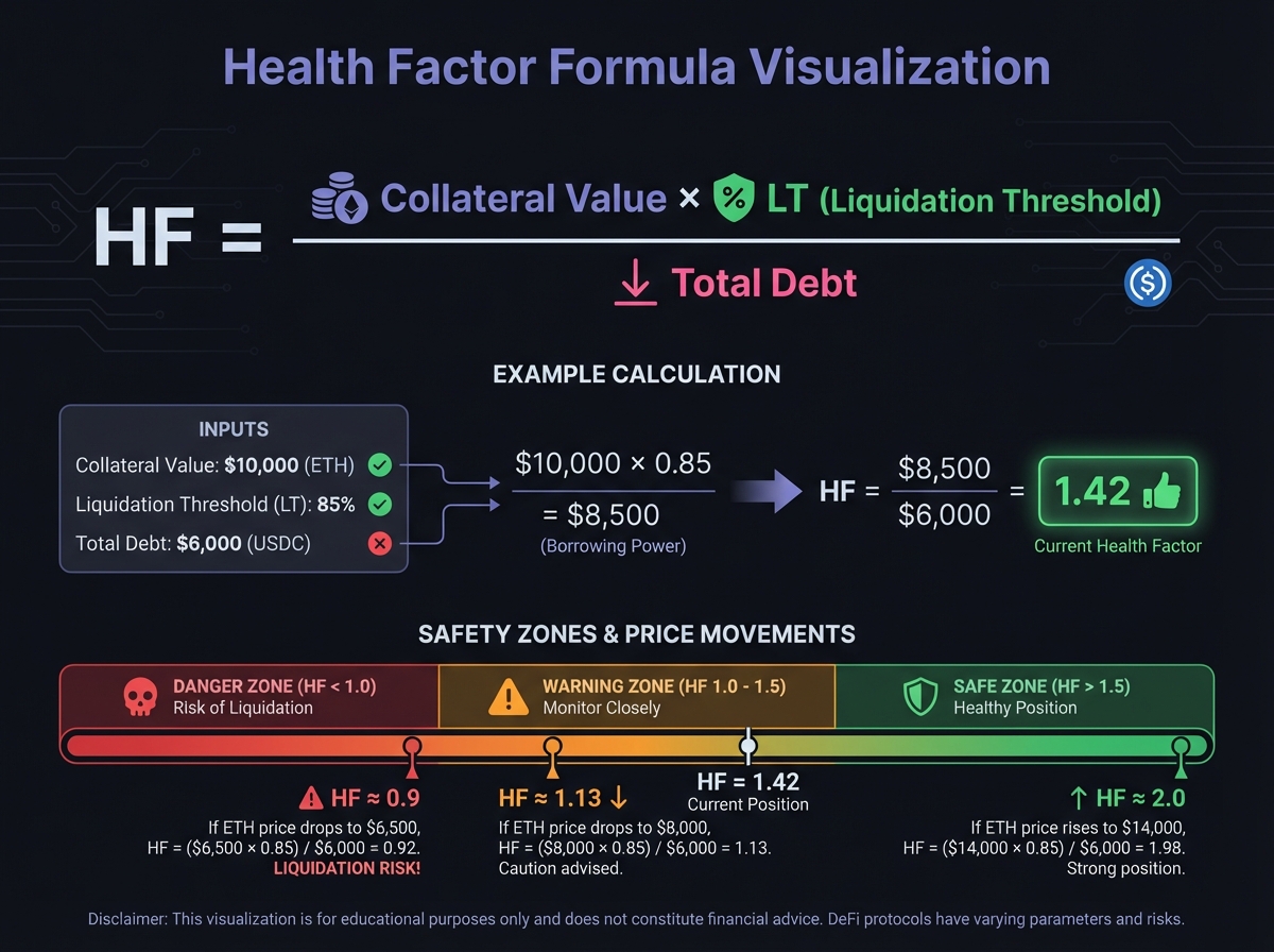
$$Health Factor = \frac{Collateral Value \times Liquidation Threshold}{Total Debt}$$

Interpreting Health Factor

HF > 1.0: Position is safe

• HF = 2.0: Can withstand ~50% collateral price drop
• HF = 1.5: Can withstand ~33% collateral price drop
• HF = 1.1: Danger zone—any small price movement risks liquidation

HF ≤ 1.0: Position is liquidatable

• HF = 1.0: Exactly at liquidation threshold
• HF < 1.0: Position is underwater (should have been liquidated)

Strategic Health Factor Targets

For Beginners: HF > 2.0

• Provides substantial buffer against volatility
• Allows you to sleep at night
• Reduces stress and monitoring frequency

For Active Traders: HF = 1.5 - 2.0

• Higher capital efficiency
• Requires active monitoring
• Acceptable for experienced users

Danger Zone: HF < 1.3

• High liquidation risk
• Requires constant vigilance
• Not recommended for beginners

Calculating Health Factor: Step-by-Step

Scenario: You deposit ETH and borrow USDC

Initial Position:

• Collateral: 5 ETH @ $2,000/ETH = $10,000
• Borrowed: $6,000 USDC
• Liquidation Threshold: 85%

Health Factor Calculation: $$HF = \frac{$10,000 \times 0.85}{$6,000} = \frac{$8,500}{$6,000} = 1.42$$

Interpretation: HF = 1.42 means the collateral can drop ~30% before liquidation.

What Happens if ETH Drops to $1,500?

• New collateral value: 5 ETH × $1,500 = $7,500
• Debt remains: $6,000 (plus accrued interest)
• New HF = ($7,500 × 0.85) ÷ $6,000 = $6,375 ÷ $6,000 = 1.06

Status: Still safe but approaching danger zone. You should consider adding collateral or repaying debt.

Health Factor with Multiple Collaterals

When you have multiple collateral types, the formula aggregates:

$$HF = \frac{\sum(Collateral_i \times LT_i)}{Total Debt}$$

Example:

• Collateral 1: 3 ETH @ $2,000, LT = 85% → $5,100 effective
• Collateral 2: $4,000 USDC, LT = 90% → $3,600 effective
• Total Debt: $7,000 USDC

$$HF = \frac{$5,100 + $3,600}{$7,000} = \frac{$8,700}{$7,000} = 1.24$$

💧 Utilization Rate and Interest Rate Curves

What is Utilization Rate?

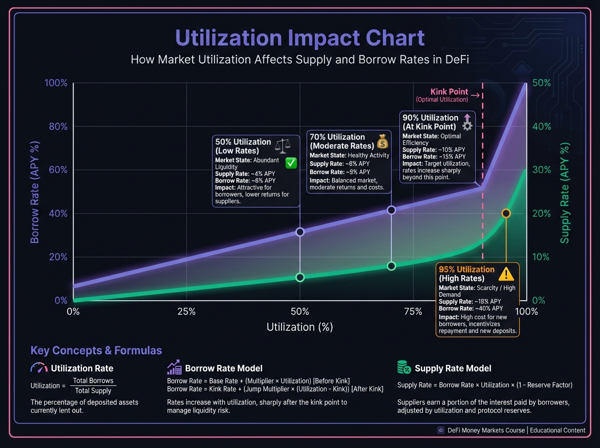
Utilization Rate (U) = The percentage of supplied assets currently borrowed:

$$U = \frac{Total Borrowed}{Total Supplied} \times 100%$$

Example:

• Pool has 100 USDC supplied
• 60 USDC is borrowed
• Utilization = 60 ÷ 100 = 60%

Why Utilization Matters

Utilization directly drives interest rates through the interest rate model:

• Low utilization (< 50%): Lower rates (less demand, more supply)
• Medium utilization (50-80%): Moderate rates (balanced)
• High utilization (> 80%): Higher rates (high demand, low supply)
• Very high utilization (> 90%): Extremely high rates (liquidity crisis warning)

The "Kinked" Interest Rate Model

Most protocols use a kinked curve with two distinct phases:

Phase 1: Below the Kink (e.g., U < 90%)

• Linear or gentle slope
• Supply rate: 2-5% APY
• Borrow rate: 5-8% APY
• Stable and predictable

Phase 2: Above the Kink (U > 90%)

• Exponential spike
• Supply rate: 10-50%+ APY
• Borrow rate: 50-200%+ APY
• Designed to incentivize repayments

Example: Interest Rate Curve

Below Kink (U = 70%):

• Supply rate: 4% APY
• Borrow rate: 6% APY
• Spread: 2% (to protocol reserves)

At Kink (U = 90%):

• Supply rate: 5% APY
• Borrow rate: 8% APY
• Spread increases

Above Kink (U = 95%):

• Supply rate: 15% APY
• Borrow rate: 50% APY
• Massive spread to attract liquidity

The Liquidity Freeze Risk

Critical Risk: If utilization reaches 100%, lenders cannot withdraw until borrowers repay.

Example Scenario:

• Pool has $1M USDC supplied
• $1M USDC borrowed
• Utilization = 100%
• You try to withdraw $10,000
• Result: Transaction fails—no liquidity available

Protection Mechanisms:

• Interest rate spikes incentivize repayments
• High rates attract new deposits
• Reserve funds (if protocol has them)
• Utilization caps (max borrowing limits)

📊 Interest Rate Calculations

How Supply Rates Work

When you lend assets, you earn interest based on:

1. Utilization rate (how much is borrowed)
2. Borrow rate (what borrowers pay)
3. Reserve factor (protocol's cut)

Simplified Formula: $$Supply Rate = Borrow Rate \times Utilization \times (1 - Reserve Factor)$$

Example:

• Borrow rate: 8% APY
• Utilization: 75%
• Reserve factor: 10% (protocol keeps 10%)

$$Supply Rate = 8% \times 0.75 \times 0.90 = 5.4% APY$$

How Borrow Rates Work

Borrow rates are determined by the interest rate model based on utilization:

Linear Model (simplified): $$Borrow Rate = Base Rate + (Utilization \times Slope)$$

Kinked Model (most common):

• Below kink: Lower slope
• Above kink: Steeper slope (exponential)

Accrued Interest Calculation

Interest accrues continuously, not daily or monthly.

For Lenders:

• Your balance grows automatically
• aToken balance increases over time
• Compound effect: You earn interest on interest

For Borrowers:

• Your debt increases over time
• Interest compounds
• Must repay principal + accrued interest

Example: Borrowing $10,000 at 6% APY:

• After 1 month: Debt = $10,000 × (1 + 0.06/12) = $10,050
• After 6 months: Debt = $10,000 × (1 + 0.06/2) = $10,300
• After 1 year: Debt = $10,000 × 1.06 = $10,600

Key Insight: If you don't monitor your position, the debt grows even if collateral price stays the same.

🔮 The Role of Oracles

What Are Oracles?

Oracles are bridges between off-chain price data and on-chain smart contracts. They feed real-world price information (like ETH/USD) to the protocol.

Oracle Types

1. Chainlink (Push-Based)

• Updates pushed to chain regularly
• Industry standard for Ethereum
• Highly secure and reliable
• Updates every few hours or minutes

2. Pyth Network (Pull-Based)

• Updates on-demand when needed
• Used for high-frequency chains (Solana, Sui)
• Lower latency for fast transactions
• More efficient for high-throughput networks

3. Redstone (On-Demand)

• Pull-based oracle
• Used by some protocols for flexibility
• Can provide custom data feeds

Oracle Risk

The Risk: If an oracle provides incorrect price data, the protocol makes decisions based on wrong information.

Attack Vector: Oracle manipulation via flash loans

• Attacker takes large flash loan
• Manipulates price on low-liquidity DEX
• Oracle reads manipulated price
• Protocol liquidates positions incorrectly
• Attacker profits from liquidations

Protection Mechanisms:

• Multiple oracle sources (e.g., Chainlink + Uniswap TWAP)
• Price staleness checks (reject old prices)
• Confidence intervals (require price consensus)
• Circuit breakers (pause if price moves too fast)

Why Oracle Choice Matters

Different protocols use different oracles, which affects risk:

Chainlink: Most secure, but updates may lag during volatility Pyth: Fast updates, good for high-frequency chains TWAP: Smooths out manipulation but may lag behind market

For Beginners: Prefer protocols using established oracles (Chainlink) with multiple data sources.

🧮 Complete Calculation Example

Let's work through a complete example:

Initial Position Setup:

• You deposit: 10 ETH @ $2,000/ETH = $20,000 collateral
• Protocol parameters:
  • LTV: 75%
  • Liquidation Threshold: 80%
  • Interest: 5% APY borrow rate

Step 1: Calculate Maximum Borrow

• Max borrow = $20,000 × 0.75 = $15,000

Step 2: Decide Borrowing Amount

• You borrow: $10,000 USDC (conservative, 50% of max)

Step 3: Calculate Initial Health Factor $$HF = \frac{$20,000 \times 0.80}{$10,000} = \frac{$16,000}{$10,000} = 1.60$$

Step 4: After 6 Months

Scenario A: ETH Price Stable

• Collateral: Still 10 ETH @ $2,000 = $20,000
• Debt: $10,000 × (1 + 0.05/2) = $10,250
• New HF = ($20,000 × 0.80) ÷ $10,250 = 1.56

Scenario B: ETH Rises 25%

• Collateral: 10 ETH @ $2,500 = $25,000
• Debt: $10,250
• New HF = ($25,000 × 0.80) ÷ $10,250 = 1.95 ✅ Safer

Scenario C: ETH Drops 30%

• Collateral: 10 ETH @ $1,400 = $14,000
• Debt: $10,250
• New HF = ($14,000 × 0.80) ÷ $10,250 = 1.09 ⚠️ Danger zone

Analysis:

• Scenario A: Position safe, slight HF decline from interest
• Scenario B: Position safer, can borrow more or enjoy buffer
• Scenario C: Must take action—add collateral or repay debt

🎓 Beginner's Corner: Common Math Mistakes

Mistake 1: Confusing LTV with liquidation threshold

• Wrong: "LTV is 80%, so I'll get liquidated at 80%"
• Right: Liquidation occurs at the LT (often 85%), not LTV

Mistake 2: Ignoring accrued interest

• Wrong: "My debt stays the same"
• Right: Debt grows continuously. A 5% APY borrow rate means ~0.42% monthly increase

Mistake 3: Not accounting for price volatility

• Wrong: "ETH won't drop 50%"
• Right: Crypto is volatile. A 50% drop in a day is possible. Calculate HF at worst-case scenarios

Mistake 4: Misunderstanding utilization

• Wrong: "High utilization means I earn more" (true but risky)
• Right: High utilization means higher rates but also higher risk of liquidity freezes

Mistake 5: Not monitoring Health Factor

• Wrong: "I'll check it monthly"
• Right: Monitor daily or use alerts. Prices can move fast, and interest accrues continuously.

🔬 Advanced Deep-Dive: Dynamic Interest Rates

Adaptive Interest Rate Models

Some protocols (like Morpho) use adaptive curves that adjust automatically:

Target Utilization: The protocol targets a specific utilization (e.g., 90%)

Mechanism:

• If utilization > target: Curve shifts up, rates increase
• If utilization < target: Curve shifts down, rates decrease
• This maintains consistent utilization levels

Formula (simplified): $$Borrow Rate = Base + (Utilization - Target) \times Sensitivity$$

Result: Markets maintain high utilization (efficient capital use) while keeping rates reasonable.

Compounding Frequency

Interest can compound at different frequencies:

Continuous Compounding (most DeFi):

• Interest accrues every block
• Formula: $A = P \times e^{rt}$
• Most accurate representation

Block-by-Block:

• Interest calculated per block
• Updates continuously
• Standard for on-chain protocols

Daily Compounding:

• Interest calculated daily
• Less accurate but simpler
• Rare in modern DeFi

📈 Real-World Calculation: Aave USDC Market

Market State:

• Total Supplied: $500,000,000 USDC
• Total Borrowed: $350,000,000 USDC
• Utilization: 70%

Interest Rates (at 70% utilization):

• Supply APY: 4.5%
• Borrow APY: 6.5%
• Spread: 2% (to Aave reserves)

Your Position:

• You supply: $10,000 USDC
• Daily earnings: $10,000 × 0.045 ÷ 365 = $1.23/day
• Monthly earnings: $1.23 × 30 = $37/month
• Annual earnings: $450/year

If Utilization Spikes to 95%:

• Supply APY: 12% (estimated)
• Borrow APY: 45% (estimated)
• Your new daily earnings: $10,000 × 0.12 ÷ 365 = $3.29/day

Trade-off: Higher yields but increased risk of liquidity freeze if utilization hits 100%.

🔧 Interactive Tools

Interactive Health Factor Calculator

Practice calculating Health Factor, LTV, and liquidation prices with this interactive tool:

Launch Lending Borrowing Calculator →

🔑 Key Takeaways

1. LTV vs LT: LTV is maximum borrowing; LT is liquidation trigger—they're different!
2. Health Factor is your safety score—keep it > 1.5 (ideally > 2.0)
3. Utilization drives rates: High utilization = high yields but high risk
4. Interest accrues continuously: Debt grows even if prices don't move
5. Oracles are critical: Wrong prices lead to wrong liquidations
6. Monitor regularly: Prices and interest change constantly

🚀 Next Steps

Now that you understand the mathematics, Lesson 3 will show you the risks in detail—liquidation mechanics, how to protect yourself, and what to avoid.

Complete Exercise 2 to practice these calculations and build your mathematical intuition.

Remember: Math protects your capital. Master these formulas, and you'll make informed decisions. Ignore them, and you'll risk liquidation or miss profitable opportunities.

← Back to Summary | Next: Exercise 2 → | Previous: Lesson 1 ←